

With the release of version 4.0.1, NSX introduced support for stateful services on T0 or T1 gateway running in Active-Active topologies. Prior to NSX 4.0.1, configuration of stateful services required to have the gateways configured in Active-Standby mode. The reason for this was asymmetric routing as the return path for traffic can be on a different edge node compared to forward traffic. With NSX 4.0.1, a new routing methodology based on IP hashing and traffic punting was introduced which will ensure that both forward and return traffic and handled by the same edge node. Stateful Active-Active services also introduces newer terminologies like interface groups, edge sub-clusters, shadow / peer-shadow interfaces, traffic punting etc which we will cover in this multi-part blog series. We will also see new flow patterns for Northbound, Southbound and East-West traffic compared to previous stateless active-active and active-standby configuration.
Not all stateful services are supported in the initial release. The below features are currently available:
- Gateway firewall (L4 and L7)
- IDS/IPS
- URL Filtering
- TLS inspection
- NAT
We also have few supported T0-T1 topologies for stateful active-active services which we will cover later. In this four part blog series we will break down the contents as below:
Part 1 : Single tier stateful Active-Active T0 gateway
Part 2 : Two tier stateful Active-Active T0 gateway (with stateful Active-Active T1 gateway attached)
Part 3 : Routing considerations and Packet walks
Part 4 : Edge Sub-clusters and failure domains
Let’s get started:
Single Tier stateful Active-Active T0 gateway
Below is the T0 Active Active Stateful topology which we we have set up in our homelab.

This topology has:
- One Tier 0 gateway configured in Active-Active stateful mode.
- Tier 0 gateway is deployed on an edge cluster with four (4) edge nodes.
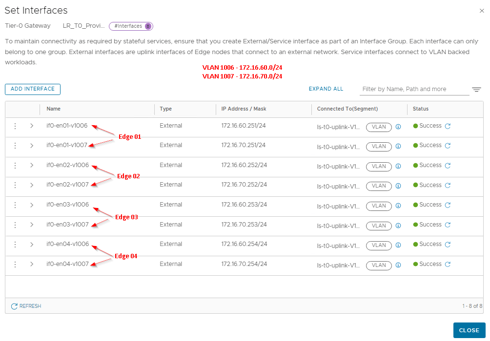
- Total of eight (8) T0 uplink external interfaces (two per edge node) over VLANs 1006 and 1007
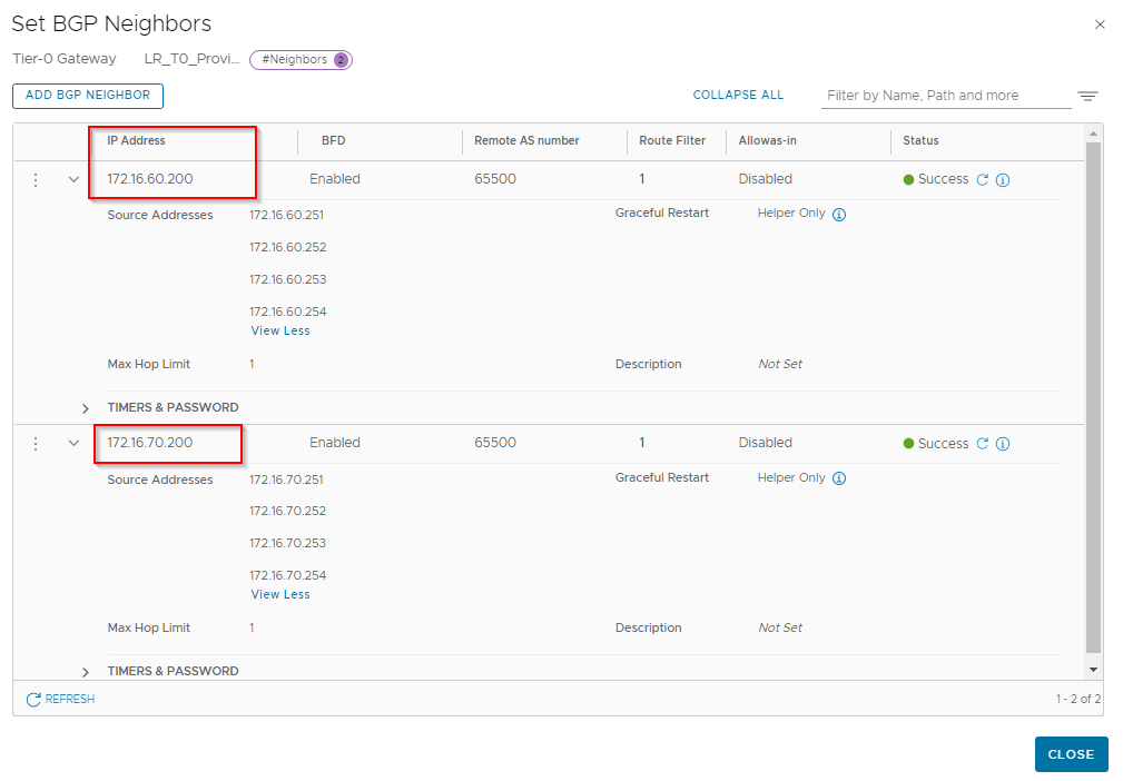
- eBGP peering established to the Leaf switches (Mikrotik router in our case) on VLAN 1006 and 1007
- Two workload segments attached to the T0 gateway (LS-DevApps01 and LS-StgApps)
- Route redistribution enabled with network reachability to the workload segments
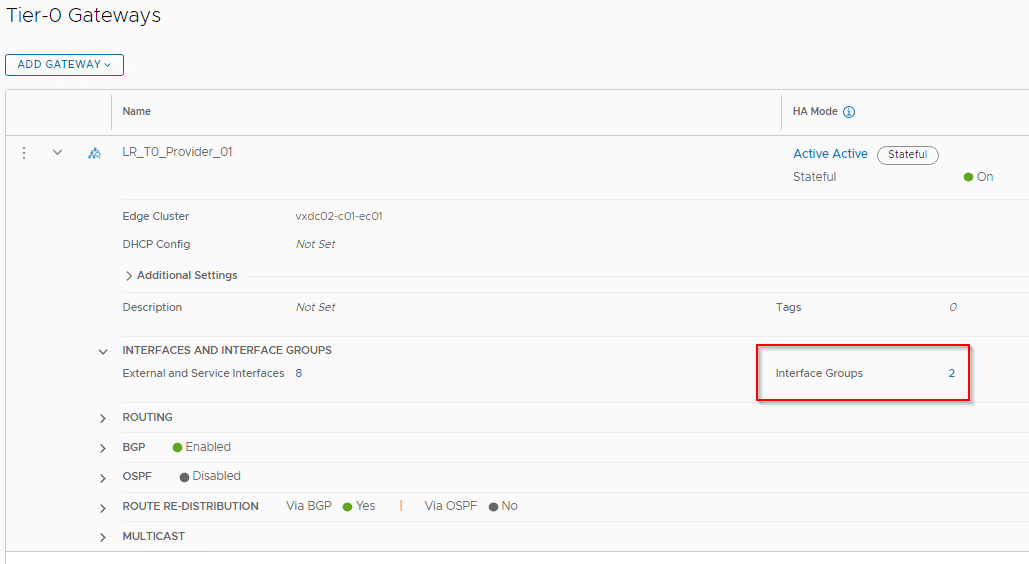
The configuration is pretty much same with regards to our traditional Active-Active or Active-Standby gateway configuration but with few additional settings which we will discuss below.


At this moment, this is how our T0 SR topology looks like (taken from NSX topology viewer).

Now, with regards to routing:
- This is a single tier routing with logical segments attached directly to T0 gateway
- T0 DR construct is available on the edge transport nodes and on all the ESXi transport nodes where the logical segments are realized.
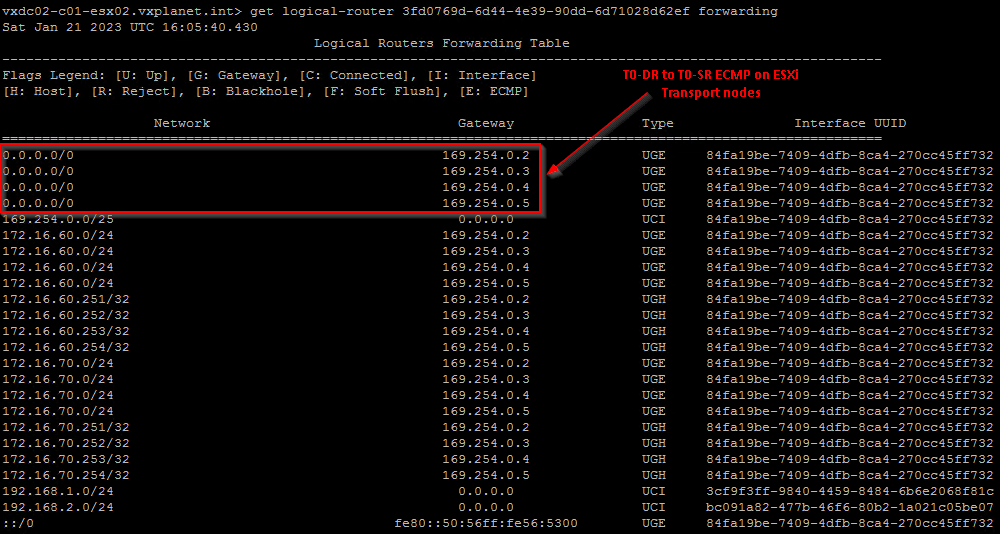
- There is T0 DR to T0 SR ECMP (four paths) on all the ESXi transport nodes.
- Edge nodes always prefer local forwarding. ie, T0 DR next hops to T0 SR on the same edge node.
- Northbound traffic egresses out of the T0 SR uplinks over VLAN 1006 and 1007 (uplink ECMP)
Below is the T0 DR next hops (ECMP) from an ESXi transport node. Notice the four ECMP paths northbound.
Below is the T0 DR next hop from the edge nodes.

So far what we saw as pretty much same with regards to the routing methodology we dealt previously. If you are interested to learn more about the traffic patterns and ECMP, please check out my three-part blog series which I did a while back.
Part 1: https://vxplanet.com/2019/10/26/nsx-t-tier1-sr-placement-and-the-effect-on-northbound-ecmp-part-1/
Part 2: https://vxplanet.com/2019/10/28/nsx-t-tier1-sr-placement-and-the-effect-on-northbound-ecmp-part-2/
Part 3: https://vxplanet.com/2019/10/28/nsx-t-tier1-sr-placement-and-the-effect-on-northbound-ecmp-part-3/
With stateful Active-Active services, we now have additional routing between edges (also called traffic punting) in order to support stateful flows. This traffic punting is based on a hashing algorithm based on IP address to select an edge node who will be authoritative for holding the stateful information for the specific flow. The hash is based on destination IP address of the packet if the flow is northbound and is based on source IP address if the flow is southbound. Once an edge node is selected based on the hash value, traffic for the specific flow will punt to this edge node for forwarding to next hop. In order to support this, we have some additional terminologies which we will cover one by one:
- Edge sub-clusters
- Interface groups
- Shadow interfaces
- Peer-shadow interfaces
- Punt logical segments (system)
Edge sub-clusters
Edge sub-cluster is a logical cluster created within the edge cluster which consists of a pair edge nodes. This edge pair will always be in sync with each other with regards to stateful information. For a specific stateful flow, one edge node within the edge cluster will be active and the other node will be standby and will take over when the primary edge node fails. There can be only 2 edge nodes within the edge sub-cluster, and this selection is made automatically while the T0 stateful active-active gateway is initialized. For this reason, we should always scale edge clusters with even number of nodes.
In an event where we have odd number of nodes, an edge sub-cluster will be created with a single node and any stateful information in this sub-cluster will not have redundancy.
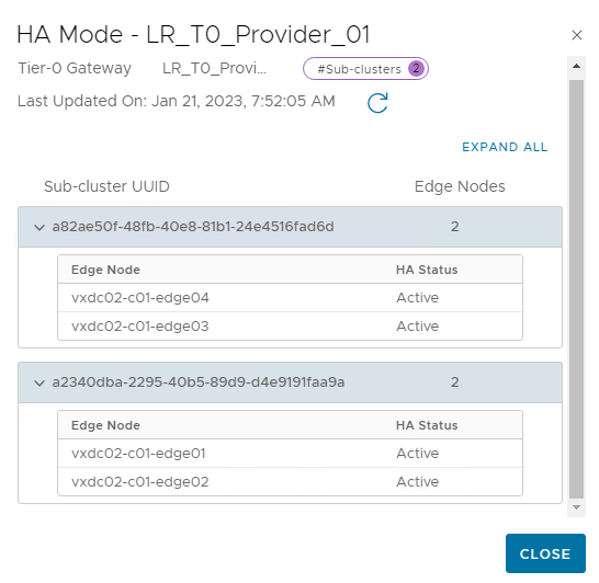
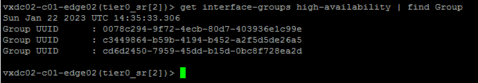
High availability status of edge SRs will now display sub clusters to which they are a member of. We can see edge 1 and edge 3 are part of separate edge sub-clusters.


In an event where we loose both edge nodes within a sub-cluster, we loose all the stateful information in the sub-cluster and the flow needs to be re-initiated. A new sub-cluster will then be chosen for the flow.
Interface groups
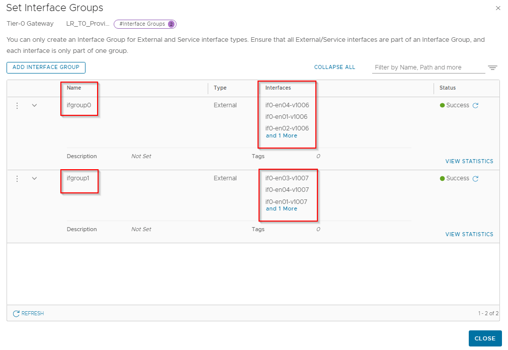
Interface groups are a way to organize or group together similar interfaces which would require the same stateful policies (firewall or nat). Interface groups can be created based on edge specific requirements like uplink VLAN membership, internet / DMZ etc. In our topology above, we have three interface groups created – two manually by us for the T0 uplink interfaces and one by the system for the T0 SR – DR backplane interface.
- Interface Group 0 (IFG0) – This has four interfaces (one from each edge node) which are the T0 uplink external interfaces on VLAN 1006. This is manually created
- Interface Group 1 (IFG1) – This has four interfaces (one from each edge node) which are the T0 uplink external interfaces on VLAN 1007. This is manually created
- Interface Group (System) – This has four interfaces (one from each edge node) which are the T0 SR – DR backplane interfaces (IntraTier transit link ports) attached to system generated transit logical segment. This is automatically created and managed by the system.
Stateful policies attached to interfaces (T0 uplinks for example) will be protected only if they are a part of interface group. Once an interface is added to interface group, system will create a shadow interface and peer-shadow interface which we will cover next.
The following conditions apply while creating interface groups:
- Only one interface from an edge SR can become a part of an interface group. For eg: if there are two T0 uplink interfaces, we will require two interface groups.
- One interface can be a part of only one interface group. It can’t be added to two interface groups
- We can’t mix and match interface types. ie, we can’t add external interfaces and service interfaces to a same interface group.
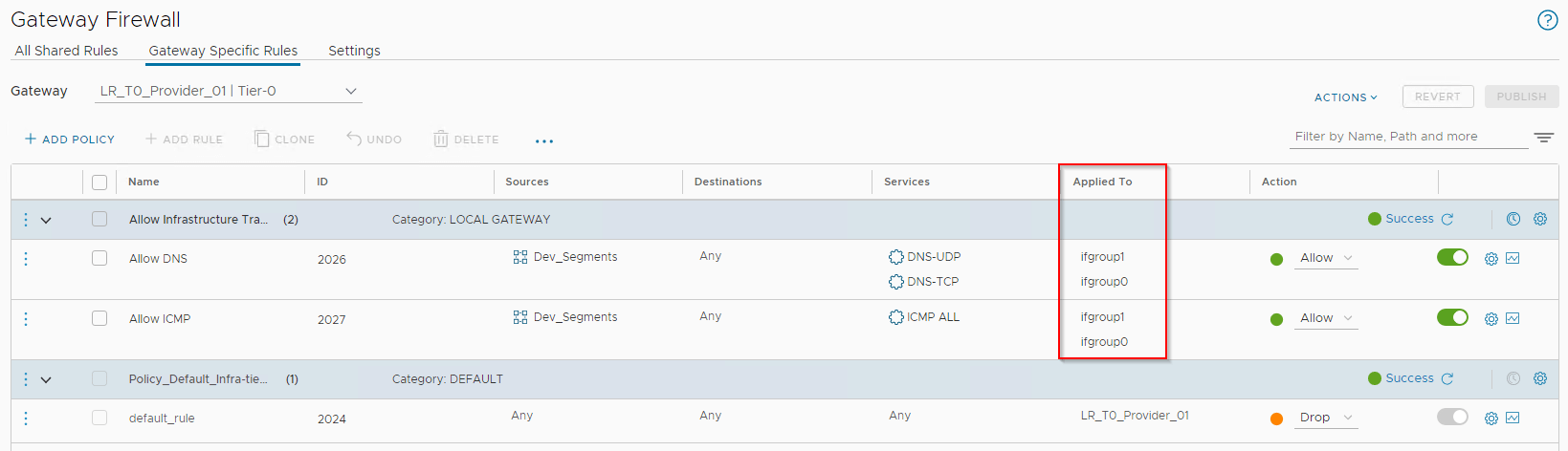
While creating stateful policies (firewall or NAT), the policies are applied to interface groups so that the interfaces are protected.
Below is a physical view of the interface groups for T0 SR uplink interfaces. Note that a shadow interface and peer-shadow interface is automatically plumbed in once an uplink interface is added to the interface group.

Below is the logical view of an interface group with respect to policy enforcement. Policies are applied to interface groups as if it is applied on a regular interface.

Below is the interface group which is created by the system for the TO SR-DR backplane interface. Shadow and peer-shadow interfaces are plumbed in for the backplane interfaces as well.

Below is the interface group configuration from our topology.
Interface groups has to be configured symmetrical across the edge nodes. Below is the cli output from two edge nodes.

Shadow and peer-shadow interfaces
Whenever an interface is added to an interface group (uplinks, service interface or backplane ports), a shadow port is created for that specific interface. This shadow port is assigned with a unique mac address and is linked to the original interface as the master interface. This shadow interface is attached to a system generated punt logical segment which spans across all the edge nodes in the edge cluster. Any traffic that needs to be punted to a different edge node will be sent across this shadow interface. Mac addresses of shadow interfaces of all the edge nodes will be kept in sync with each other. This punt mac address table is queried based on the IP hash that is generated whenever a flow hits an edge node. For an S -> N (northbound) flow, the shadow interface of T0 SR – DR backplane interface is used to punt traffic to the respective edge that holds the stateful information. Similarly for an N -> S (southbound) flow, the shadow interface of T0 SR uplink interface (V1006 or V1007) is used to punt traffic to the respective edge that holds the stateful information.
Shadow interfaces are always in operational UP status.
For each shadow interface there is a peer-shadow interface which is basically a backup interface to handle punted traffic of the peer edge node in case of peer edge failure. This peer-shadow interface has a mac address same as the shadow interface of the peer edge node. This peer-shadow interface is also attached to the same punt logical segment where the shadow interfaces are attached.
The peer-shadow interface is in operationally DOWN status and will come up only if peer edge node failure is detected.
The below sketch shows the shadow and peer-shadow interfaces for an interface (uplink or backplane) which is added to an interface group. Traffic is punted through the shadow interface over the punt logical segment (shown below).

Now let’s verify the shadow interfaces, peer-shadow interfaces and shadow-macs using cli of edge nodes.
T0 External interface on VLAN 1006
We can see that the shadow macs are in sync across all the edge nodes for the external interface.


We see shadow and peer-shadow interfaces created on all edge nodes for the external interface.


T0 External interface on VLAN 1007
We can see that the shadow macs are in sync across all the edge nodes for the external interface.


We see shadow and peer-shadow interfaces created on all edge nodes for the external interface.


TO SR – DR Backplane interface
We can see that the shadow macs are in sync across all the edge nodes for the T0 SR- DR backplane interface.


We see shadow and peer-shadow interfaces created on all edge nodes for the T0 SR – DR backplane interface.


Punt logical segment
Punt logical segment is a system generated VNI to carry punted traffic between edges over the shadow interfaces and peer-shadow interfaces (in case of failure scenarios). This punt LS will be realized only on edge transport nodes and not on any ESXi transport nodes.

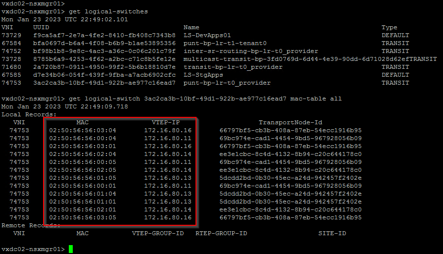
As mentioned earlier, mac addresses of shadow interfaces are in sync with all the edge nodes. As such, we see mac address of all the three shadow interfaces of each edge node in the mac-address table of the punt LS.

Determining the edge node for traffic flows
For northbound traffic (S -> N), edge node is selected based on a hash value using destination IP address. This IP hashing is performed as soon as the traffic reaches the backplane interface of T0 SR construct of an edge node. For eg: if the calculated IP hash value selects edge 3 while the traffic reached edge 2, the traffic is punted to edge 3 over the shadow interface for the backplane interface. This happens at layer 2 by modifying the destination mac address of the packet to point to the shadow interface of edge 3. Once traffic reaches edge 3, all northbound lookup happen locally and state information is added or updated accordingly.
Similarly for southbound traffic (N -> S), edge node is selected based on a hash value using source IP address. This IP hashing is performed as soon as the traffic reaches the T0 SR uplink interface of an edge node. If this is a return traffic for an existing flow, hash value using the source IP address will return the same value and as such, the same edge node who has the stateful information for the forward flow is selected. This is true as long as the source IP is not modified. Traffic is punted over to the correct edge node through the shadow interface of T0 SR uplinks over layer 2. All southbound lookup now happens locally until the traffic is tunneled to the ESXi transport node.
Lets test this. We will find out which edge node is selected for northbound flow based on few destination IP addresses, for eg: 8.8.8.8 and 172.16.10.50
We see Edge 3 is selected for destination 8.8.8.8 and
Edge 1 is selected for destination 172.16.10.50


Next, we will find out which edge node is selected for southbound flow (or return flow) for the same IP addresses. Note that for southbound traffic, IP hash is based on source IP address.
We see Edge 3 is selected for source 8.8.8.8 and
Edge 1 is selected for source 172.16.10.50


Since the same edge node handles both forward and return traffic, statefulness of the flow is achieved.
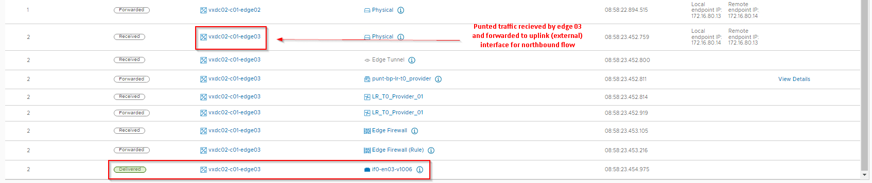
Let’s do a traceflow and confirm this. We see that for destination 8.8.8.8, traffic has been punted to edge 3 (as expected).

Creating stateful policies
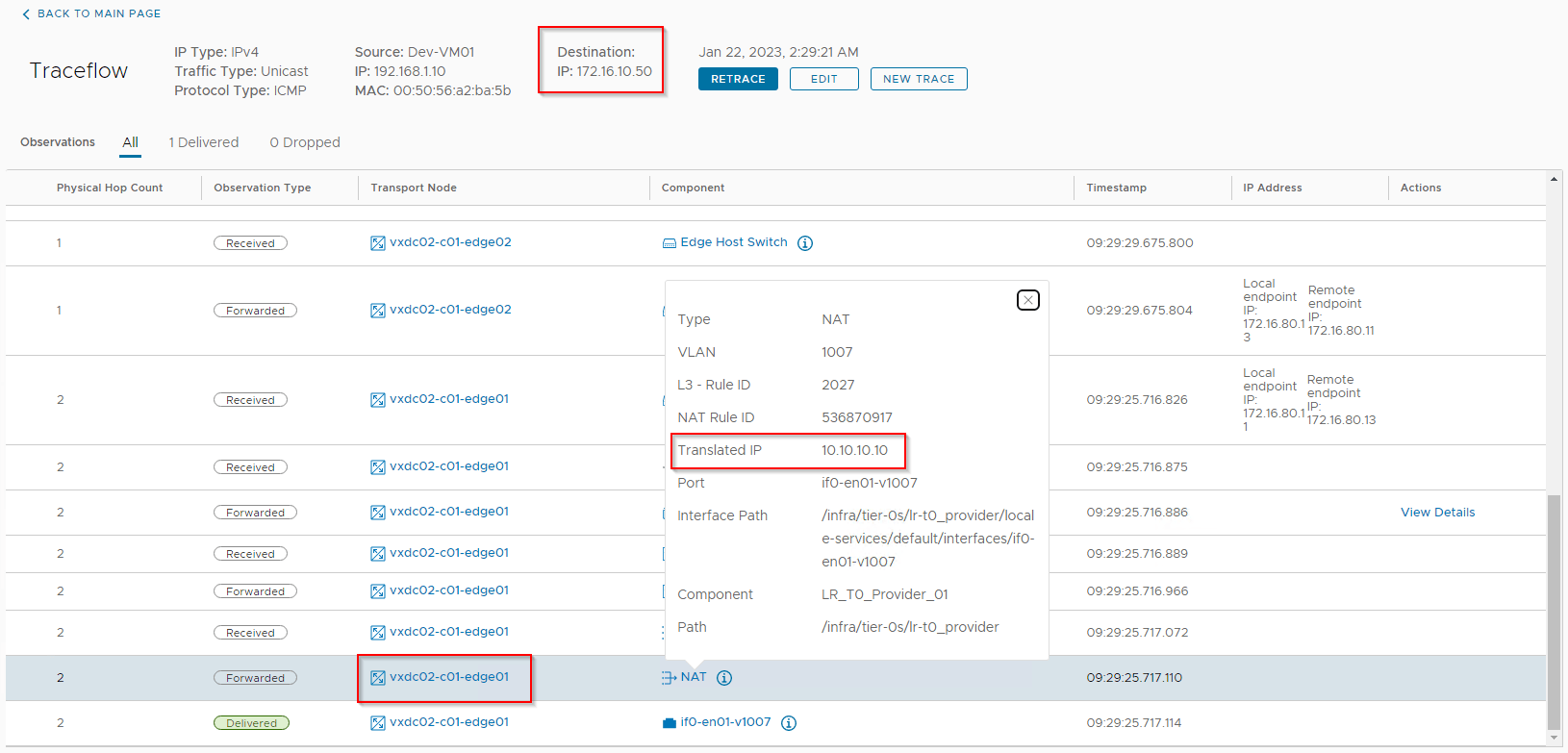
Now lets create few gateway firewall and SNAT policies and verify the traffic flow using NSX Traceflow.
Note that we applied the policies to interface groups to achieve active-active statefulness. If the policy is applied to an individual interface instead, they wont be protected.


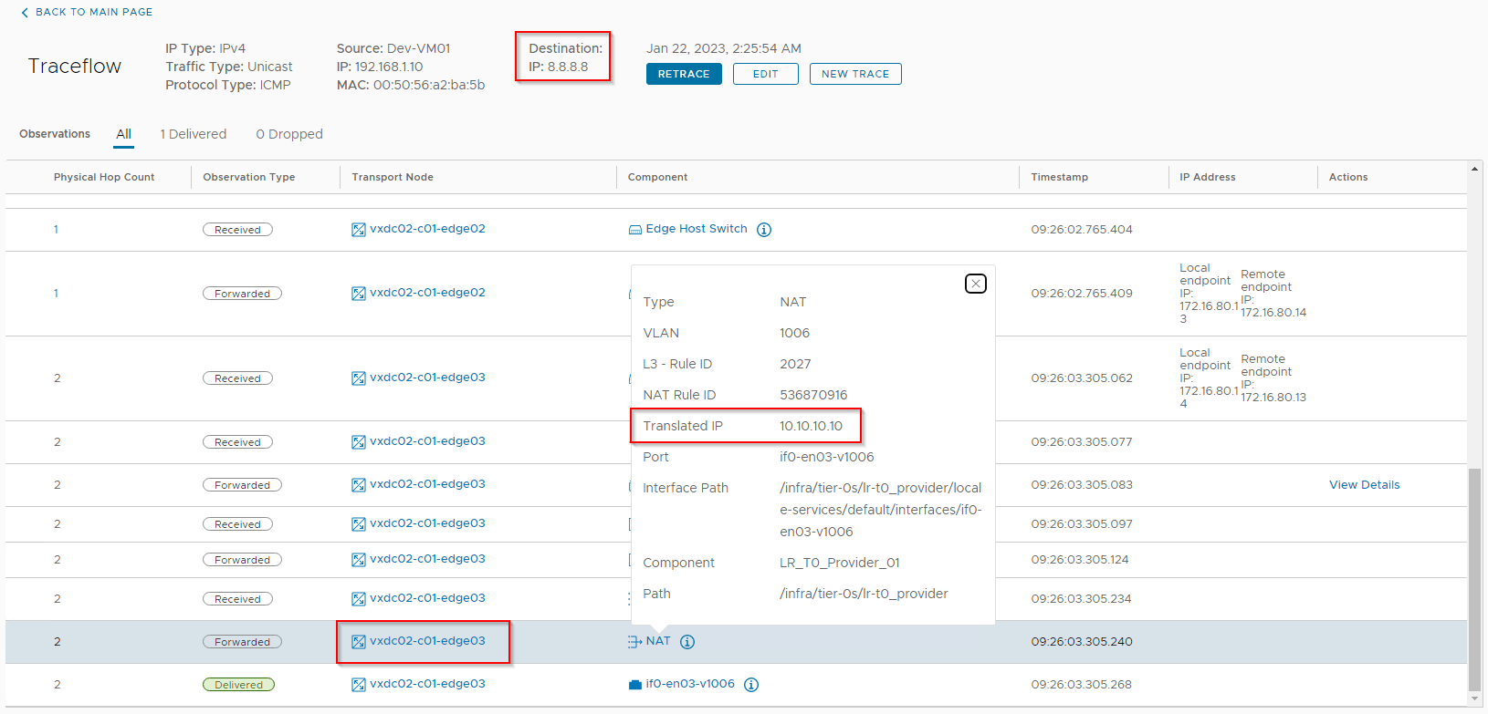
Traceflow shows that edge 3 is selected for destination 8.8.8.8 and edge 1 is selected for destination 172.16.10.50 (as expected)
This has been a lengthy article, now it’s time to break and have a coffee 🙂
If you would like to understand more, please refer the official documentation below:
We will meet in Part 2 where we deal with two tier routing by attaching a stateful Active-Active Tier 1 gateway downstream. Stay tuned!!!
I hope the article was informative. Thanks for reading.
Continue reading? Here are the other parts of this series:
Part 2 : https://vxplanet.com/2023/01/30/nsx-4-0-1-stateful-active-active-gateway-part-2-two-tier-routing/
One thought on “NSX 4.0.1 Stateful Active-Active Gateway – Part 1 – Single Tier Routing”